Examples

The following examples are illustrative of real world problems that are easily solved by using MATLink to get the best of both MATLAB and Mathematica.

Fast Delaunay triangulations

Mathematica has a DelaunayTriangulation function in the ComputationalGeometry package, but it is very slow. (It does have its strong points though, such as the capability to use exact arithmetic and deal with collinear points.) Using MATLink, we can use MATLAB's delaunay function to compute the Delaunay triangulation of a set of points as

delaunay = Composition[Round, MFunction["delaunay"]];

Since Mathematica's function returns a vertex adjacency list, we'll need to post-process the output to compare it with MATLAB's:

Needs["ComputationalGeometry`"];
delaunayMma[points_] :=
	Module[{tr, triples},
		tr = DelaunayTriangulation[points];
		triples = Flatten[
			Function[{v, list},
				Switch[Length[list],
				 (* account for nodes with connectivity 2 or less *)
				 1, {},
				 2, {Flatten[{v, list}]}, _, {v, ##}& @@@ Partition[list, 2, 1, {1, 1}]]
			] @@@ tr, 1];
		Cases[GatherBy[triples, Sort], a_ /; Length[a] == 3 :> a[[1]]]
	]

A random set of points will usually have a unique Delaunay triangulation, so we can test that the two systems return identical results

pts = RandomVariate[NormalDistribution[], {100, 2}];
Sort[Sort /@ delaunay[pts]] === Sort[Sort /@ delaunayMma[pts]]

and plot the triangulations with

trianglesToLines[t_] :=
  Union@Flatten[{{#1, #2}, {#2, #3}, {#1, #3}} & @@
	  Transpose[Sort /@ t], {{1, 3}, {2}}];
Graphics@GraphicsComplex[pts, Line@trianglesToLines@delaunay[pts]]

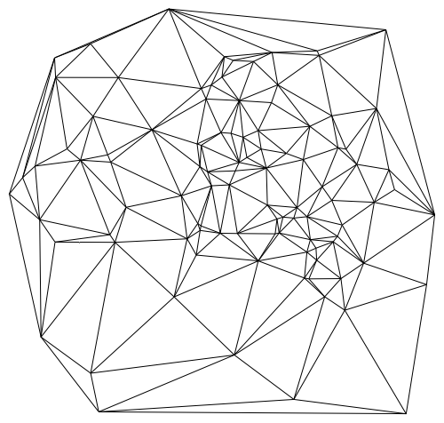
Not only is delaunay much faster than DelaunayTriangulation (especially for larger data sets), it is also much faster than the triangulator used internally by ListDensityPlot. Hence we can use MATLAB's delaunay to design a custom listDensityPlot which is faster than the built-in function and can handle large data sets as follows:

Options[listDensityPlot] = Options[Graphics] ~Join~ {ColorFunction -> Automatic, MeshStyle -> None, Frame -> True};

listDensityPlot[data_?MatrixQ, opt : OptionsPattern[]] :=
	Module[{in, out, tri, colfun},
		tri = delaunay[data[[All, 1;;2]]];
		colfun = OptionValue[ColorFunction];
		If[Not@MatchQ[colfun, _Symbol | _Function], Check[colfun = ColorData[colfun], colfun = Automatic]];
		If[colfun === Automatic, colfun = ColorData["LakeColors"]];
		Graphics[
			GraphicsComplex[data[[All, 1;;2]],
				GraphicsGroup[{EdgeForm[OptionValue[MeshStyle]], Polygon[tri]}],
				VertexColors -> colfun /@ Rescale[data[[All, 3]]]
			],
			Sequence @@ FilterRules[{opt}, Options[Graphics]], Method -> {"GridLinesInFront" -> True}
		]
	]

Let's now test our custom function against the built-in function for 30000 points:

pts = RandomReal[{-1, 1}, {30000, 2}];
values = Sin[3 Sqrt[#1^2 + #2^2]] & @@@ pts;

listDensityPlot[ArrayFlatten[{{pts, List /@ values}}], Frame -> True] // AbsoluteTiming
(* 0.409001, --Graphics-- *)

ListDensityPlot[ArrayFlatten[{{pts, List /@ values}}]] // AbsoluteTiming
(* 12.416587, --Graphics-- *)

The speedup is indeed quite significant. For hundreds of thousands of points, the built in ListDensityPlot is practically unusable, while listDensityPlot finishes in seconds.

When benchmarking MATLink, it's necessary to use AbsoluteTiming, which measures wall time. Timing only measures the CPU time consumed by the Mathematica kernel; it does not measure the time used by MATLAB.

Filtering sound using the signal processing toolbox

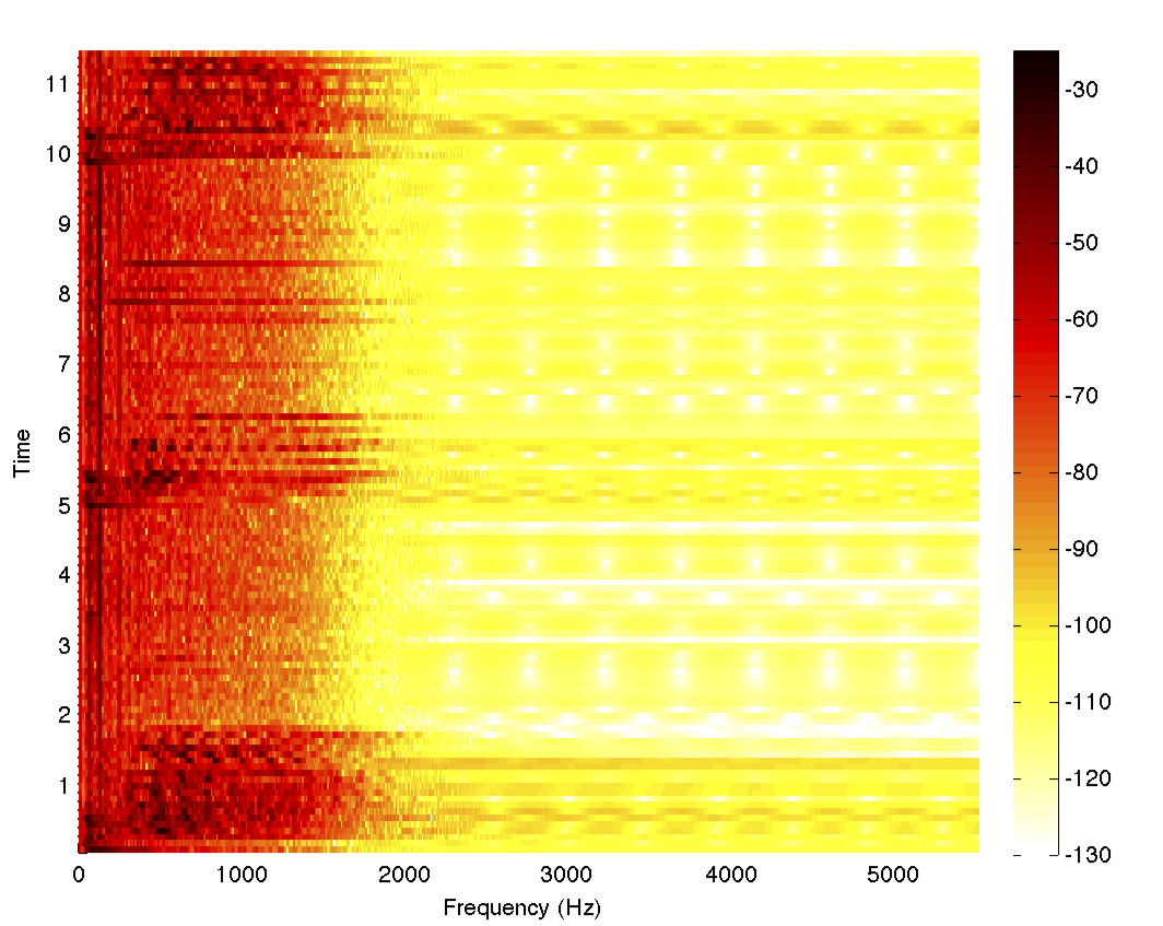
Signal processing functionality was notoriously missing from Mathematica until version 9, and still lags behind MATLAB's toolbox in terms of functionality and ease of use. Let's suppose we wanted to inspect the frequency content of an audio file and filter it (assume you're using Mathematica 8 and don't have the newer functions).

{data, fs}  = {#[[1, 1, 1]], #[[1, 2]]} &@ExampleData[{"Sound", "Apollo13Problem"}];
spectrogram = MFunction["spectrogram", "Output" -> False]; (* Use MATLAB's spectrogram *)
spectrogram[data, 1000, 0, 1024, fs]

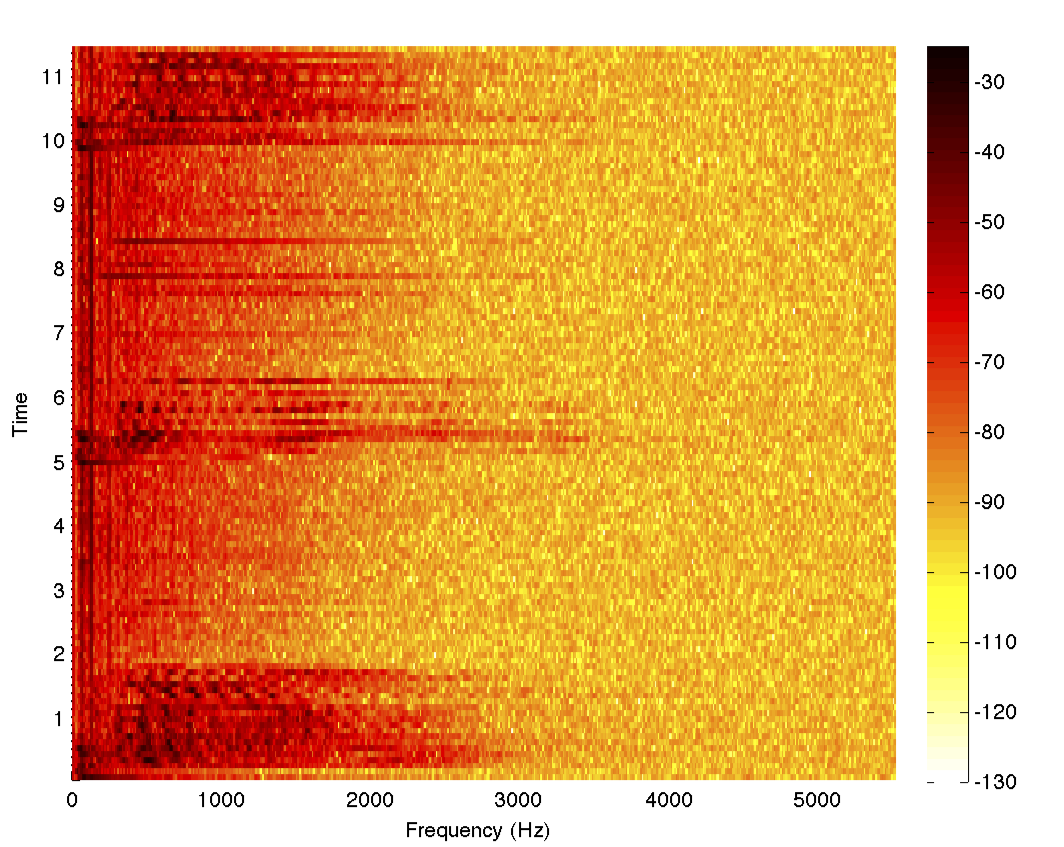
Clearly, the frequency content is mostly below 2.5 kHz, and so we can design a lowpass filter in MATLAB and also make a helper function that will return the filtered data

MSet["fs", fs];
MEvaluate["
	[z, p, k] = butter(6, 2.5e3/fs, 'low') ;
	[sos, g]  = zp2sos(z, p, k)            ;
	Hd        = dfilt.df2tsos(sos, g)      ;
"]
filter = MFunction["myfilt", "@(x)filter(Hd,x)"];

Now we're all set to use the filter function from within Mathematica on the data. This simple example demonstrates how one can fill in for missing functionality. It saves us the trouble of having to develop a complicated filter design algorithm in Mathematica (which is not an easy task) and spend hours debugging it. The code for the Butterworth filter could've come from anywhere — the file exchange or Stack Overflow or previously written code or perhaps even, as in this case, an example from the documentation for butter. A slight tweak of the parameters to suit the needs at hand, and we're good to proceed with our work in Mathematica.

To complete the example, let's filter the data using our filter and look at the spectrogram

filteredData = filter@data;
spectrogram[filteredData, 1000, 0, 1024, fs]

For fun, we can also play both the filtered and unfiltered data and listen to the differences

ListPlay[data, SampleRate -> fs]
ListPlay[filteredData, SampleRate -> fs]